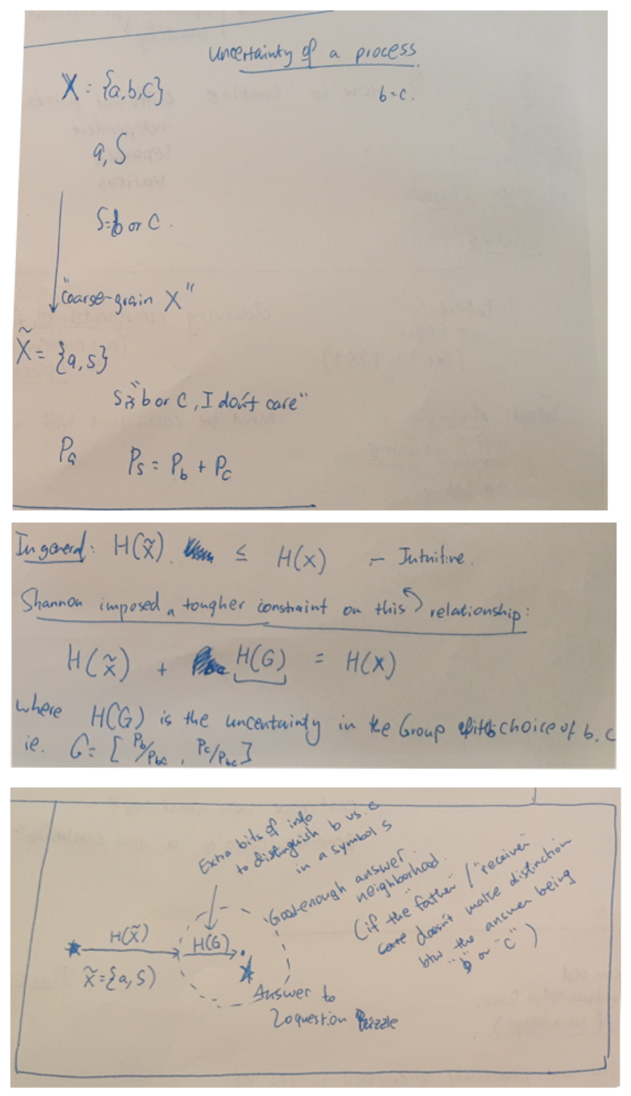
One of the axioms in Shannon's information theory is that (Shannon's) entropy satisfies coarse-graining property:
While reading Information Theory for Intelligent People by S.DeDeo
This property is closely related to the conditional probabilities.
In communication -- regardless of the types of agents involved, eg. between the people over a phone, between parent cell's DNA to daughter cell's DNA, between a disk storage at time T and that at time T+10), or between me (the writer of this article) and you (the reader),
there is some 'tolerance' bound that allows "good-enough" intention/semantics to be transmitted and understood between the sender and the receiver.
How is this idea related to the Rate-Distortion theory or error-correcting codes?
Can this idea help us understand/define the "semantic" information (vs. Shannon's Information measure is often called "syntactic" because it is ignorant/invariant to the identities of the events whose probabilities within the process we are measuring the uncertainty of).
Pondering...
Coarse-graining/level of details when describing a process
As we 'abstract' away from particular representational form of an event/instance, we move from semantics+form domain to → → → semantics+less form domain. This allows me to say "The chair is blue" and you understand what general color the chair is.
At which level of abstraction / this ladder of coarse-graining, do we get sufficient (ie. good-enough to communication our intentions) level of semantics?
If we measure $H(\tilde{X})$ at that level, can we say that quantity measures 'semantic information'?
The difference $H(G)$ is the force/gradient that drives the flow of information -- information of what?
For example, in geometric case, \(\mu(A)\) can be interpreted as a (physical) length (if \(A\) is one dimensional), mass (if \(A\) is two dimensional), or volumn (if three-dim) of a region \(A\). In the case that \(\mu\) is a measure of probability, \(\mu(A)\) is the probability mass of event, "random variable \(X\) takes values in the set \(A\) (also called event \(A\))"
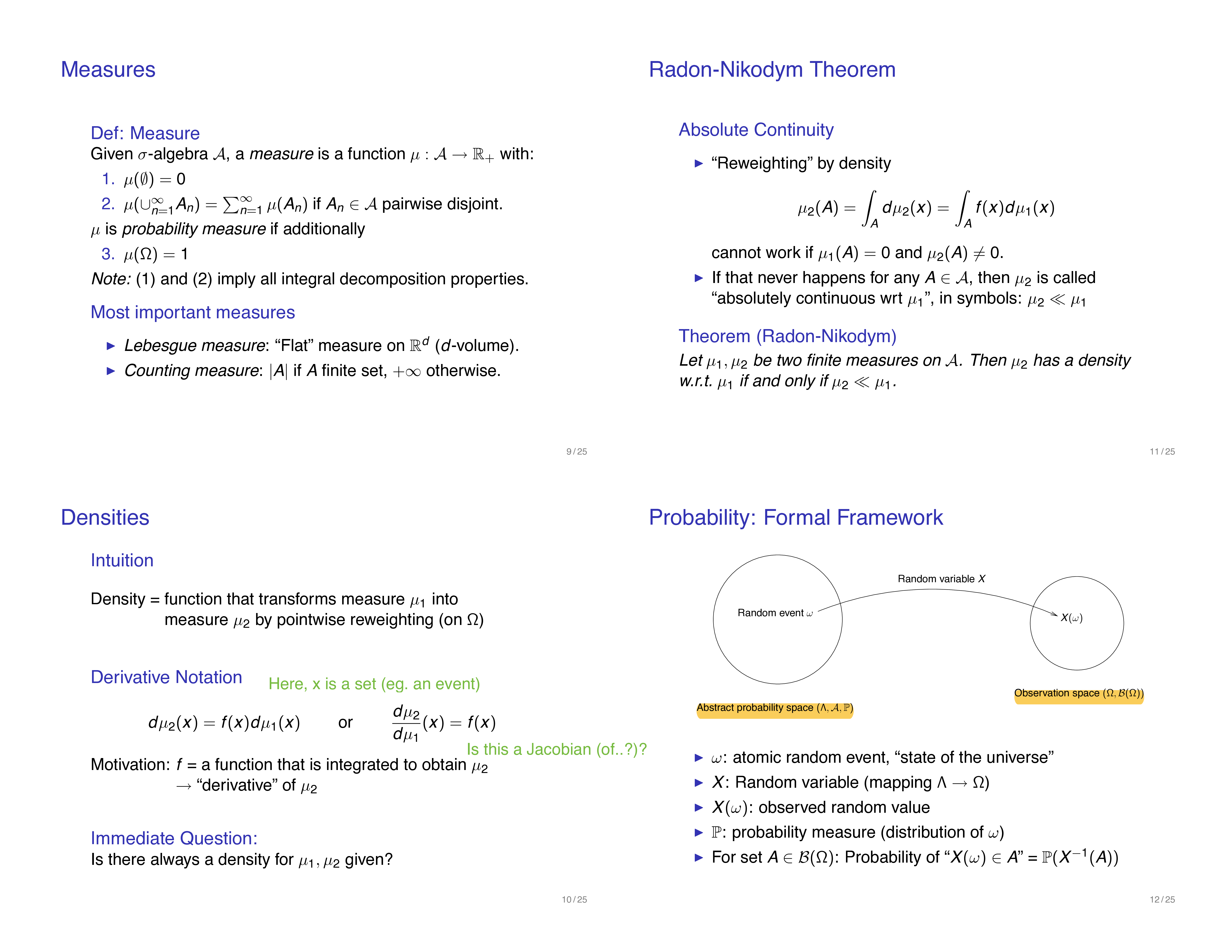
Density
A (probability) density is a function that transforms one measure to another measure by pointwise reweighting (on the abstract sample space \(\Omega\))
Measure-theoretic formalism for Probability
abstract probability space vs. observation space
Think of the abstract probability space as the entire system of the universe. A point in the space is a state of the universe (eg. a long vector of values assigned to all existing atoms' states). We often don't have a direct access to this "state", ie. it is not fully observable to us. Instead we observe/measure variables that are some functions of this atomic configuration/state (\(w\)). This mapping from a state of the universe to a value that the variable of our interest is observed/measured to take is called a "Random Variable".
Random Variable
- is a function that maps a outcome in the abstract probability space's sample space \(\Lambda\) to the sample space of the observation space \(\Omega\) (often \(\mathbb{R}\))
- it is the key component that connects the abstract probability space (which we don't get to directly observe) to the observation space
- Image measure \(\mu_{X}\) is the (derived/induced) measure on the observation space that is related to the abstract probability space via the random variable \(X\).
- We need it since the measure on the abstract probability space \(\mathbb{P}\) is not known explicitly, but we need to have a way to descirbe the measure of sets in the Borel set of the observation space.
- To assign measures to an event in the observation space, we use "Image measure" \(\mu_{X}\) which is linked to \(\mathbb{P}\) via:
$$ \mu_{X}(A) := \mathbb{P}(X^{-1}(A))$$
- In other words, we compute the probability measure of an event \(A\) (ie.the probability that the random variable X takes a value in the set A) by:
1. Map the set A in the observation space to a space in the abstract probability space, \(A^{\leftarrow} = X^{-1}(A)\)
2. Compute the probability of event \(A^{\leftarrow}\) using \(\mathbb{P}\)
Relationship between two random variables and their image measures
"Density" describes the relationship between two random variables and their image measures:
Source
Theoretical Foundations of Nonparametric Bayesian Models, by P.Orbanz. MLSS2009: video part 1, 2. Slides 1, 2 Great introduction of measure theory just as much in detail to be relevant for statistics (and nonparametric Bayesian models)
Lec on VAE, by Ali Ghodsi: This lecture motivates KL Divergence as the measurement of difference in the average information content of two random varialbes, whose distributions are \(p\) and \(q\) in in the article.
Wiki: It clears up different terminologies that are (misused) to refer to the KL.
It gives a great example of "answering 20 questions" problem as a way to think about basic concepts in info theory, including entropy, KL divergence and mutual information.
\(H(X)\) is equal to the average length of an arbitrary tree, which is the number of questions to get to choice \(x\)
"(Using \(H(X)\),) (f)or any probability distribution, we can now talk about "how uncertain we are about the outcome", "how much information is in the process", or "how much entropy the process has", and even measure it, in bits" (p.3)
Explaining physical phenomenon consistent with observations
Bayesian data analysis is a way to iteratively building a mathemtical description of a physical phenomenon of interest using observed data.
Setup
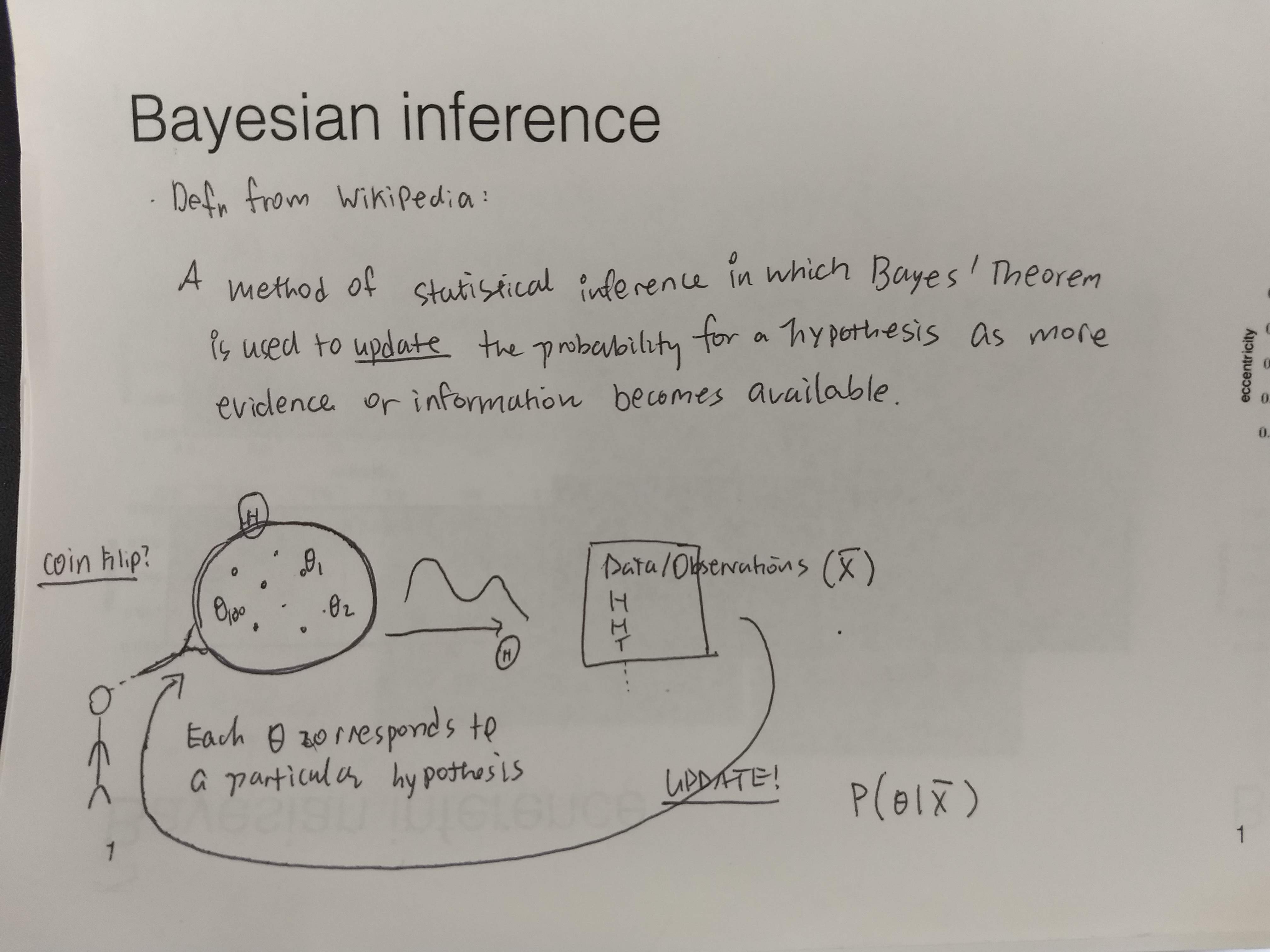
Bayesian inference is a method of statistical inference in which Bayes' Theorem is used to update the probability for a hypothesis (\(\theta\)) as more evidence or information becomes available [wikipedia].
Therefore, it is used in the following scenario. I'll refer to the workflow as the workflow of "Bayesian data analysis" following Gelman.
We have some physical phenomenon (aka. process) of interest that we want to describe with mathematical language. Why? because once we have the description (aka. mathematical model of the physical phenomenon), we can use it to explain how the phenomenon works as a function of its inner components, predict how it would behave as the inner components or its input variables take different values, (... any other usage of the mathematical model?)
We decide how to describe the phenomenon using a mathematical language by specifying:
Variables
Relations
This is the step of "choosing a model family (aka. a statistical model)"
Now we have specified a family of probability models, each of which corresponds to a particular hypothesis/explanation of the physical process of interest. What we need to do is, to choose the "best" hypothesis from all of these possible hypotheses. To do so, we need to observe how the physical phenomenon manifests by collecting data of the outcomes of the phenomenon.
Collect data of the outcomes of the phenomenon.
"Learn"/"Fit" the model to the data. (aka, "estimate" the parameters (\(\theta\)) with the data). In English, this corresponds to "find a hypothesis of the phenomenon that matches the observed data "best"". To find such hypothesis \(\theta \in \Theta\), we need to define what is means to be the "best" hypothesis given the model (aka. Hypothesis space) and the observed data. We formulate this step as an optimization problem:
choose a loss function \(L(\theta \mid \text{model}, \bar{X})\)
Solve the optimization problem of finding argmin of the loss:
$$ \theta^{*} = \arg min ~~ L(\theta \mid \text{model}, \bar{x})$$
Note: \(L(\theta \mid \text{model}, \bar{x}) \equiv L(\theta \mid \Theta, \bar{X})\). So we can rewrite the optimization objection as:
More specific scenario: a phenomenon with unobservable variables
Most physical phenomenon involves variables that we can't directly observe. These are called "Latent variables", and a statiscal model with such unobservable variables (in addition to observed/data variables) are called "Latent Variable Model". When we are focusing on the latent variable model, we often use \(Z\) as the latent variables and \(X\) as the data sample variable. That is, if we have \(N\) observation, the sample variable will be a vector of \(N\) data variables: \(X = {X_1, X_2, \dots , X_N }\). The general setup of Bayesian data analysis workflow above (ie. choose a model \(\rightarrow\) collect data \(\rightarrow\) fit the model to the data \(\rightarrow\) criticize the model \(\rightarrow\) repeat). We can express the bayesian data analysis workflow using these notations as follows:
(Note these notations are consistent with Blei MLSS2019.)
In English, describe what is the physical phenomenon of interest
Choose a statistical model by specifying
variables (nodes in the graph)
data variables (aka. observable variables): \(X\)
latent variables: \(Z\)
relations (edges in the graph)
as a (parametrized) function of its nodes
Let's denote the set of all parameters in the model, \(\theta\). Our statistical model can be expressed as: \(P(Z,X; \theta)\).
Collect data: \(\bar{X}\)
Fit the model to the observed data
Choose a loss function (a function wrt parameters): \(L(\theta;\bar{X})\) for \(\theta \in \Theta\)
Inference
Generally speaking, inference (which stems from the Philosophy of Science)
Bayesian inference method
Bayesian inference is a method of statistical inference in which Bayes' Theorem is used to update the probability for a hypothesis(\(\theta\)) as more evidence or information becomes available wikipedia.
My sketch
It is not a model, it is a general method(aka. technique, algorithm) that allows to infer unknowns probabilistically via computing, eg. marginal and conditional distributions of the model, the distribution over the parameters given observed data, the conditional distribution over the latent variables given the observed data.
Since it is a general technique (or an appoarch to doing inference) that is not tied to a specific model or a problem, we can use it whenever a suitable setup is presented. In the Bayesian Data analysis workflow, I see two places where we can use the Bayes theorem to infer some unknown quantities in the model (ie. use bayesian inference to compute unknowns given knowns).
Use bayesian inference method to learn the model from the observed data. That is, what is the probability of the parameter of the model given observation?
$$ P(\theta \mid \bar{X})$$
Use bayes' theorem to compute the conditional distribution of latent variables given observed data and a fixed parameter (eg. the learned parameter from step 1)
$$ P(Z \mid \bar{X}, \bar{\theta})$$
Note: I was living in the smog under the impression that "Bayesian inference" is tied to either 1 or 2. But now I understand "bayesian inference" just means computing probability distribution over the unknowns (either because they are unobservable (ie. conditional distribution of latent variables given observed data), or a subset of variables (ie. marginal distribution) that requires further computation on the joint distribution (aka. the probability model)). So, as Wikipedia's definition clarifies, anytime we have a quantity (with prior distribution) and make observations regarding a relevant process, we can update the prior distribution using the observed data via Bayes Theorem. That is all that is in the intimidating word "Bayesian inference". Gosh, can we please give another name to this way of doing computation with a probability model and data assumed to come from the probability model? "Inference" is such intimidating word. I feel like I need to do philosophy to use this word and everytime I hear this term, I feel like I never understand what the heck it is about because I don't understand what inference means in Philosophy. Yikes! :[
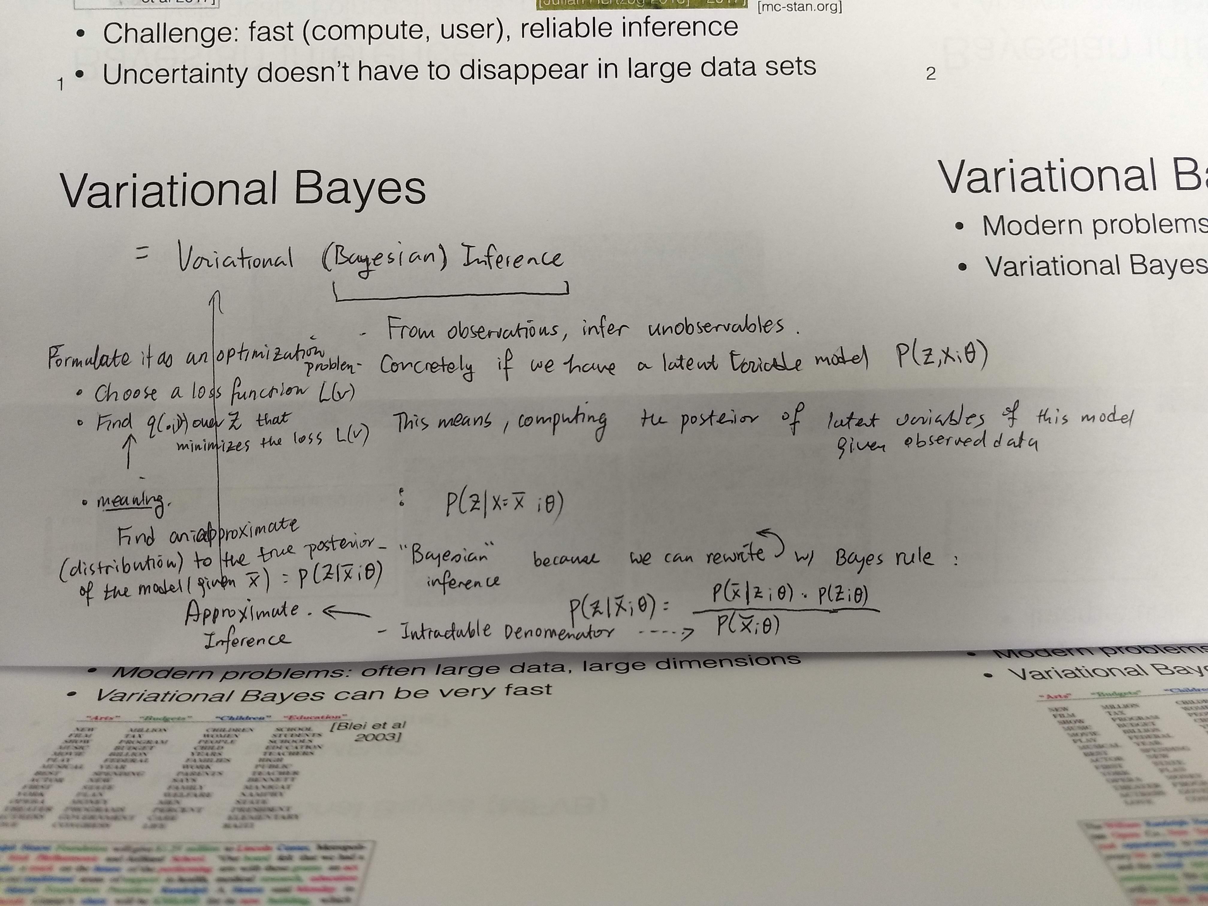
Approximate Inference
When we cannot compute the "flipped" probability ("flipped" using the Bayes Theorem) because it is, for example, too computationally expensive, we sometimes resort to an approximation of the true "flipped" probability.
Variational Approximate Inference
People call this "Variational Bayes", which I find it very loaded and unclear whether if the term refers to a method of inference or some model family because both "V" and "B" are captialized and it gives me an impressions that it's a name of some specific class of probability distributions. Yikes2! :[ Please give another name to it.
Variational Approximate Bayesian Inference is:
a method of finding a "good" approximate distribution to the "flipped" distribution of your probability model (ie. \(P\) with a fixed parameter \(\bar{\theta}\)) (ie2: "flipped" using Bayes theorem given your probability model) by formulating a proper optimization problem.
So far, we have discussed about "bayesian inference", and the need to sometimes be content with an "approximation" to the "flipped" distribution (given a fixed parameter and observed data). The last thing to understand is the "variational" part, which correpsonds to formulating the search for a "good" approximation distribution as an optimization problem. As usual for an optimization problem, we need to define "goodness", or in this case "loss"
Sketch for understanding the motivation for variational bayesian inference method (aka. Variational Bayes)
 - Intuition: roughly a measure is an integral as a function of its region
 A (probability) density is a function that transforms one measure to another measure by pointwise reweighting (on the abstract sample space
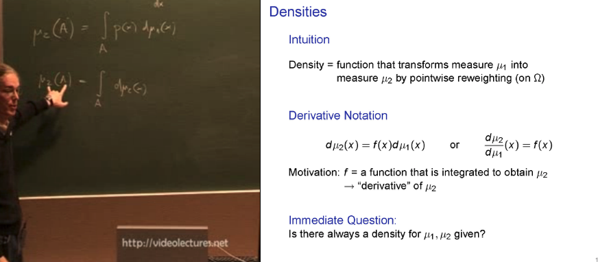
 - is a function that maps a outcome in the abstract probability space's sample space