Small Simplicity

Multimodal Distribution in Image or Text domain

Q: What does "multimodal distribution" mean in computer vision literature (eg. image-to-image translation)?

While reading papers on conditional image generation using generative modeling (eg. "Toward Multimodal Image-to-Image Translation" by Zhu et al (NIPS 2017)), I wasn't clear what was meant by "one-to-many mapping" between input image domain and output image domain, "multimodal distribution" in the output image domain, or "multi-modal outputs" (eg. Quora).

Definition

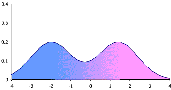
In statistics, a multimodal distribution is a continuous probability distribution with two or more modes (distinct peaks; local maxima) - wikipedia

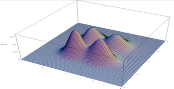
(single-variable) bimodal distribution	bivariate multimodal distribution

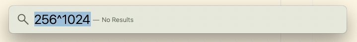
In high-dimensional space (such as an Image domain: \(P(X)\) where X lives in \(d\)-dim space where \(d\) is the number of pixels, eg. \(32x32=1024\). If each pixel \(X_i\) takes a binary value (0 or 1), the size of this image domain is \(2^{1024}\). If each pixel takes an integer value \(\in [0,255]\), then the size of this image domain is \(256^{1024}\). This, by the way, is too big to compute for Mac's spotlight:

What it means by saying "the distribution of (output) image is multimodal" is to say, there are multiple images (ie. realization of the random variable (vector) X) with the (local) maxima value of the probability. In Figure below, the green dots represent the local maxima, ie. modes of the distribution. The configurations (ie. specific values/realizations) that achieves the (local) maximum probability density are the "probable/likely" images.

So, given one input image, if the distribution of the output image random variable is multi-modal, the standard problem of

Find \(x\) s.t. \(\underset{x \in \mathcal{X}}{\arg\max} P(X)\) (\(\mathcal{X}\) is the image space)

Multimodal distribution as the distribution over the space of target domains [Domain adaption/transfer leraning]

So far, I viewed the multimodal distribution as a distribution over a specific domain (eg. Image domain), and the random variable corresponded to a realization, eg. an observed/sampled/output image instance. However,

Stochastic Thinking: Predictive non-determinism

MIT 6.0002 Lec4: Stochastic Thinking - YOUTUBE -

Often confusing categorization of a mathematical model: - SE - NB: in CS, people often use "deterministic" to mean non-randomized. This causes confusion: > "Determinism" means non-randomized. But, "Non-determinism" does not mean "randomized". - Determinism vs. Non-Determinism - ...? vs. stochastic/random - a stochastic (or random) process means,

<p hidden>![stochastic-process](images/stochastic-process.png)</p>

I think better way to put this confusion into words is: "Nondeterinistc vs. Probabilistic models" - lavalle 2006

Let's blog with Pelican

Makefile

1. make html: generates output html files from files in content folder using development config file

   • make regenerate: do make html with "listening" to new changes
   • vs. make publish: similar to make html except it uses settings in pulishconf.py

2. make serve: (re)starts a http server in the output folder. Default port is 8000

3. Go to localhost:<PORT> to see the output website
4. ghp-import -b <local-gh-branch> <outputdir>: imports content in
   to the local branch local-gh-branch

Workflow

Key points:

• Do every work in dev branch.
• Do not touch blog-build or master.
• blog-build will be indirectly modified by ghp-import (or make publish-to-github)
• and master is the branch that Github will access to show my website.
• So, manage the source (and outputs) only in dev branch.

Local dev

1. Activate the right conda env with pelican library

conda activate my-blog 

cd ~/Workspace/Blog

1. Make sure you are on dev branch git checkout dev

2. (this step is for github syncing) Add new files under content git add my-article.md

3. Generate the content with pelican make html # or, make regenerate

4. Start a local server make server

5. Open a browser and go to localhost:8000 Or whatever the port number is, set in Makefile (under the variable name of PORT)

Global dev

1. Use make publish instead of make html
2. Update the blog-build branch with contents in output folder
3. Push the blog-build branch's content to origin/master

These three steps can be done in one line:

make publish-to-github

Version control the source

Important: Write new contents only on the dev branch

git add <files> # make sure not to push the output folder

git cm "<commit message>"

git push origin dev #origin/dev is the remote branch that keeps track of blog sources

Cool Chart tool: `amcharts`

While making a visualization for my part whereabouts for the front page of this blog, I came across this easy-to-use visualization examples using amcharts. Initially, I wanted to use Google Earth Studio but it required me to import country boundaries (in KML files) as well as time to learn new toolsuites, so I find this javascript based demos more useful for my need.

List of timeline + map charts - Fishbone timeline - Fight routes on map - Flight animation on map - Timeline animation with fligh on map - and many more demos

Pretty neat!

Git refspec

Resource: git-book

Git Remotes

Remote repositories: versions of your project that are hosted on the internet

git remote -v

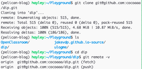
Let's say I cloned a repository from some repository, for instance git@github.com:cocoaaa/dip.git, by running:

git clone git@github.com:cocoaaa/dip.git

Then, in this cloned repo's directory in my local machine, git remote will list the shortnames of each remote handle I've specified. By default, Git gives to the server I've just cloned the shortname, origin. Use git remote -v to see both the shortname and the URLs that Git has stored for each shortname to use for reading and writing to that remote.

git remote add <shortname> <URL>

adds a remote in <URL> with the shortname of <shortname>

git fetch <remote>

The command goes out to that remote project and pulls down all the data from that remote project that I don't have yet. It does so for all branches in the remote. Upon the command execution, I should have references to all the branches from that remote, and I can merge in or inspect them at any time.

Remember that git fetch command only downloads the data to my local repository, and does NOT automatically merge it with any of my work or modify what I'm currently working on. So, it is safer than git pull, yet I'm required to merge it into my work whenever I'm ready.

For fetching and pushing, my current branch needs be set up to track a remote branch. In other words, setting up the URL to the remote repository is not enough, and we need to specify which local branch will track which remote branch.

git clone <some-repo-url> automatically sets up my local master branch to track the remote default branch (often also master) on the server I cloned from, ie. <URL>.

Push my (local) changes to the remote server (upstream)

git push <remote> <branch> pushes my local branch to my remote server. For example, if I want to push my master branch to my origin server (recall that these names are set up by git clone <some-repo-url> command automatically), run: git push origin master. Again, origin is the shortname assigned to the remote server URL, and master is the name of the local branch I'm pushing.

If I want to push my local dev-local branch to my remote repository called origin's dev-remote branch, I'd run git push origin dev-local:dev-remote. The colon syntax follows src_refspec:dst_refspec where src_refspec and dst_refspec are the refspecs of the source branch (in local) and the destination branch (in remote) of the git push action, respectively.

Q: wait, we don't need to specify which branch in the remote server to push the local branch?

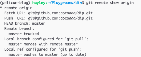
Inspecting a remote

git remote show <remote-shortname> command shows the details of the particular remote.