While making a visualization for my part whereabouts for the front page of this blog, I came across this easy-to-use visualization examples using amcharts. Initially, I wanted to use Google Earth Studio but it required me to import country boundaries (in KML files) as well as time to learn new toolsuites, so I find this javascript based demos more useful for my need.
List of timeline + map charts
- Fishbone timeline
- Fight routes on map
- Flight animation on map
- Timeline animation with fligh on map
- and many more demos
Pretty neat!
Resource: git-book
Git Remotes
Remote repositories: versions of your project that are hosted on the internet
git remote -v
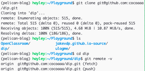
Let's say I cloned a repository from some repository, for instance
git@github.com:cocoaaa/dip.git, by running:
git clone git@github.com:cocoaaa/dip.git
Then, in this cloned repo's directory in my local machine,
git remote will list the shortnames of each remote handle I've specified.
By default, Git gives to the server I've just cloned the shortname, origin.
Use git remote -v to see both the shortname and the URLs that Git has stored for
each shortname to use for reading and writing to that remote.
git remote add <shortname> <URL>
- adds a remote in
<URL> with the shortname of <shortname>
git fetch <remote>
The command goes out to that remote project and pulls down all the data from that
remote project that I don't have yet. It does so for all branches in the remote.
Upon the command execution, I should have references to all the branches from that
remote, and I can merge in or inspect them at any time.
Remember that git fetch command only downloads the data to my local repository,
and does NOT automatically merge it with any of my work or modify what I'm currently
working on. So, it is safer than git pull, yet I'm required to merge it into my
work whenever I'm ready.
For fetching and pushing, my current branch needs be set up to track a remote
branch. In other words, setting up the URL to the remote repository is not enough,
and we need to specify which local branch will track which remote branch.
git clone <some-repo-url> automatically sets up my local master branch to
track the remote default branch (often also master) on the server I cloned from,
ie. <URL>.
Push my (local) changes to the remote server (upstream)
git push <remote> <branch> pushes my local branch to my remote server.
For example, if I want to push my master branch to my origin server (recall
that these names are set up by git clone <some-repo-url> command automatically),
run: git push origin master. Again, origin is the shortname assigned to the
remote server URL, and master is the name of the local branch I'm pushing.
If I want to push my local dev-local branch to my remote repository called origin's
dev-remote branch, I'd run git push origin dev-local:dev-remote.
The colon syntax follows src_refspec:dst_refspec where src_refspec and dst_refspec
are the refspecs of the source branch (in local) and the destination branch (in remote)
of the git push action, respectively.
Q: wait, we don't need to specify which branch in the remote server to push
the local branch?
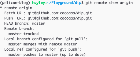
Inspecting a remote
git remote show <remote-shortname> command shows the details of the particular
remote.